Problem set 3

Short guidelines

Description

Today you will be working on a specific challenge related to quantum physics or quantum computing. In groups, your task is to develop a solution using the concepts and tools you’ve learned throughout the course. You can use any modules or libraries you find useful, such as NumPy, SciPy or QuTiP.

We will be using AI copilots to assist you in coding and problem-solving. The focus will be on collaboration, creativity, and critical thinking.

The final part of the session will involve a short presentation (15’), where each group will share their approach, solution, and reflections on the use of AI tools in their process.

Objectives

1. Understand the problem statement and requirements.

2. Collaborate with your team to brainstorm ideas and approaches.

3. Develop a solution using Python or Mathematica. You can use AI tools to assist you in coding and problem-solving.

4. Prepare a presentation to share your findings and reflect on the use of AI in your process.

Resources you can use

• Access to AI copilots/tools for coding assistance. Some examples include GenAI, ChatGPT, or other similar tools.

• Documentation and resources from previous weeks.

Short presentation outline (15’)

1. Background:

   • What was the question?

   • How did you approach it?

2. Solution development and implementation

3. Implementation (mathematical and coding)

4. Critical reflection on the use of AI copilots. Eg:

   • Which AI tool/s did you use?

   • Was it helpful, misleading, or counterproductive?

   • What resources did you need other than AI?

   • How confident are you in your solution?

   • Which parts are less clear or hard to verify?

5. Coding skills evaluation

   • To what extent do you understand the code generated with AI assistance?

   • Were there functions or code constructs used that you didn’t know before? Do you understand them now?

Problem 3

Parametrically driven Kerr model

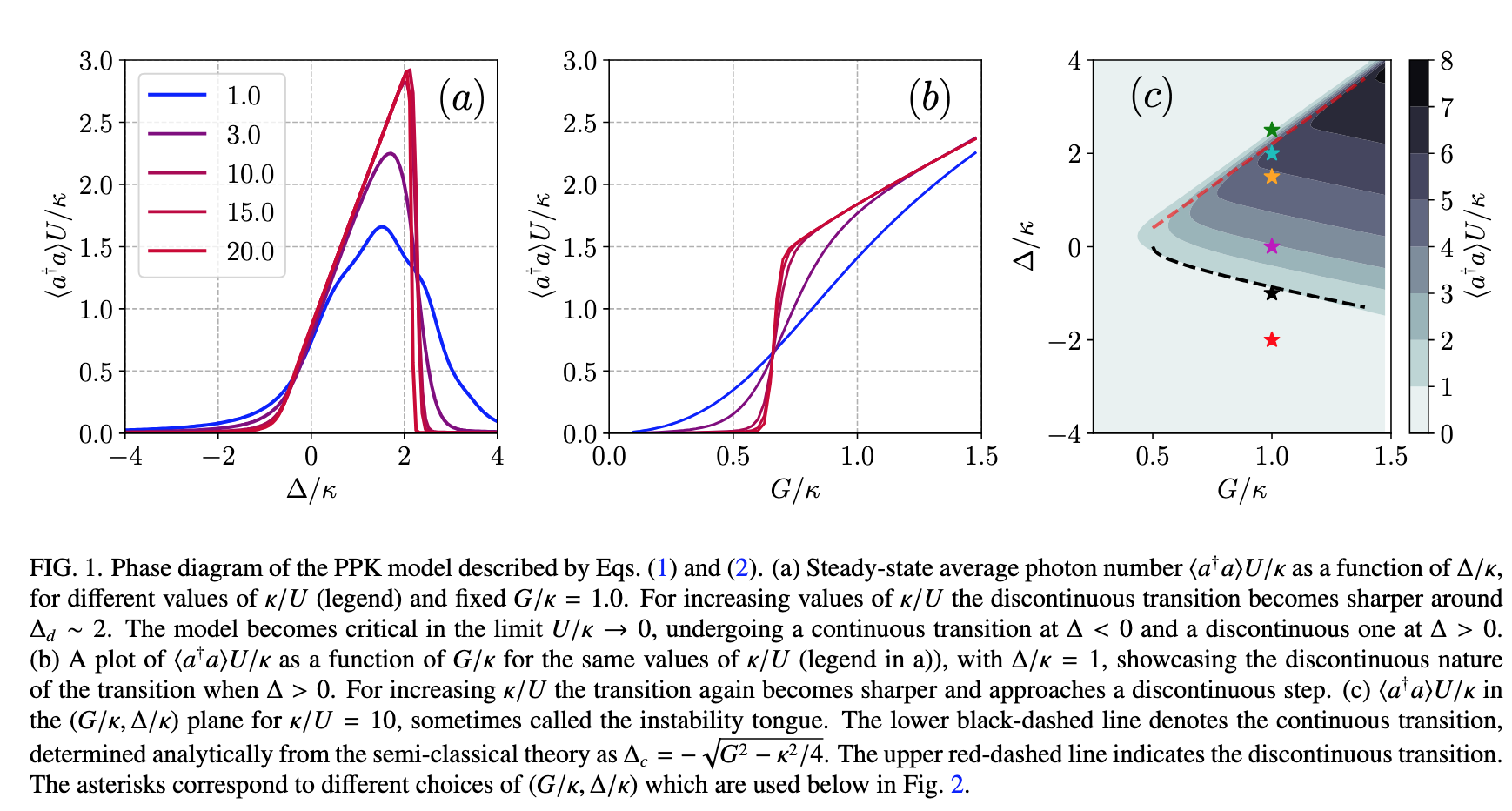
The parametrically driven Kerr model consists of a single bosonic cavity mode of frequency \(\omega_{a}\) containing a Kerr non-linearity with strength \(U\). proportional to the thrid-order nonlinear susceptibility. The cavity is parametrically driven by a pump mode at the frequency \(\omega_{p} \sim 2\omega_{a}\), which created two excitations in the cavity mode per absorbed photon. Assuming a sufficiently large separation of timescales between the cavity and pump mode dynamis, we can adiabattically eliminate the pump and describe the dynamics of the cavity mode via the interaction-picture Hamiltonian \((\hbar=1)\):

\[ \hat{H} = - \Delta \hat{a}^{ \dagger} \hat{a} + \frac{U}{2} \hat{a}^{ \dagger 2} \hat{a}^{2} + \frac{G}{2} (\hat{a}^{ \dagger 2} + \hat{a}^{2} ) \]

where \( \Delta = \omega_{a} - \omega_{p}/2 \) is the detuning of the cavity from the pump, \(G\) corresponds to the strength of the two-photon parametric pump, and \( \hat{a} (\hat{a}^{ \dagger} \) is the bosonic annihilation (creation) operator of the cavity mode satisfiying the commutation relation \( [ \hat{a}, \hat{a}^{ \dagger} ] = 1 \).

We further assume the cavity is subject to photon losses, with a loss rate \(\kappa\). As such, it can be described by the Born-Markov quantum master equation:

\[ \frac{d\hat{\rho}}{dt} = -i [ \hat{H}, \hat{\rho} ] + \kappa \left[ \hat{a} \hat{\rho} \hat{a}^{\dagger} - \frac{1}{2} \{ \hat{a}^{\dagger} \hat{a}, \hat{\rho} \} \right] \]

Task:

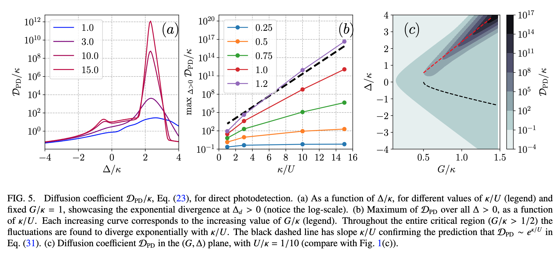
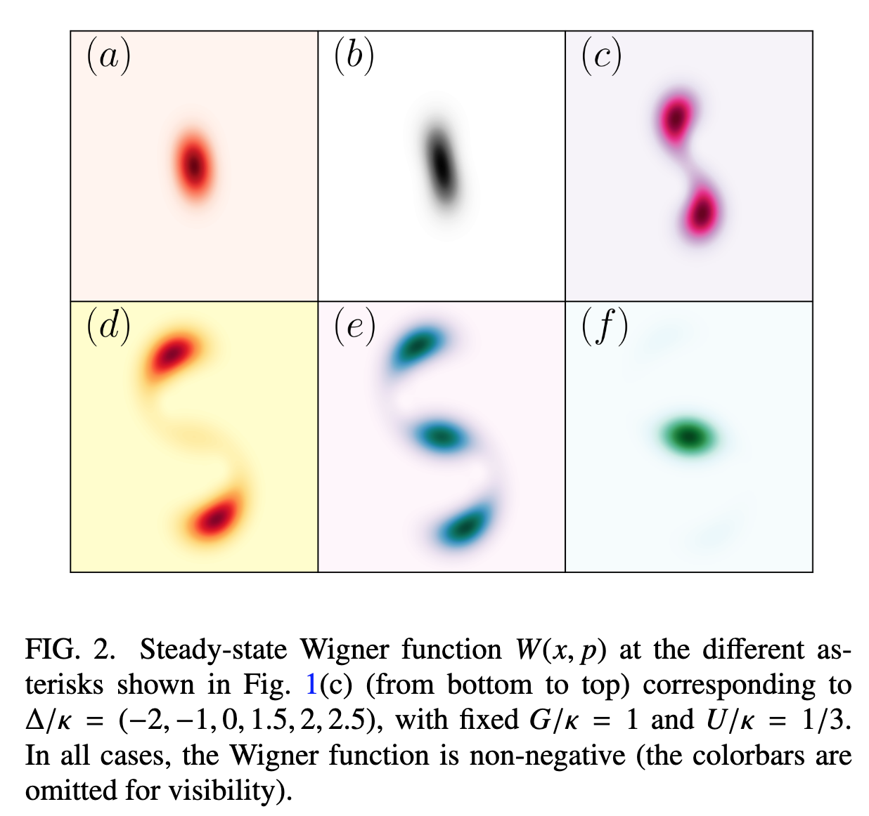
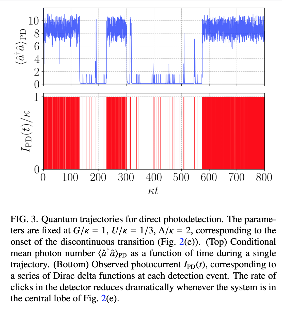
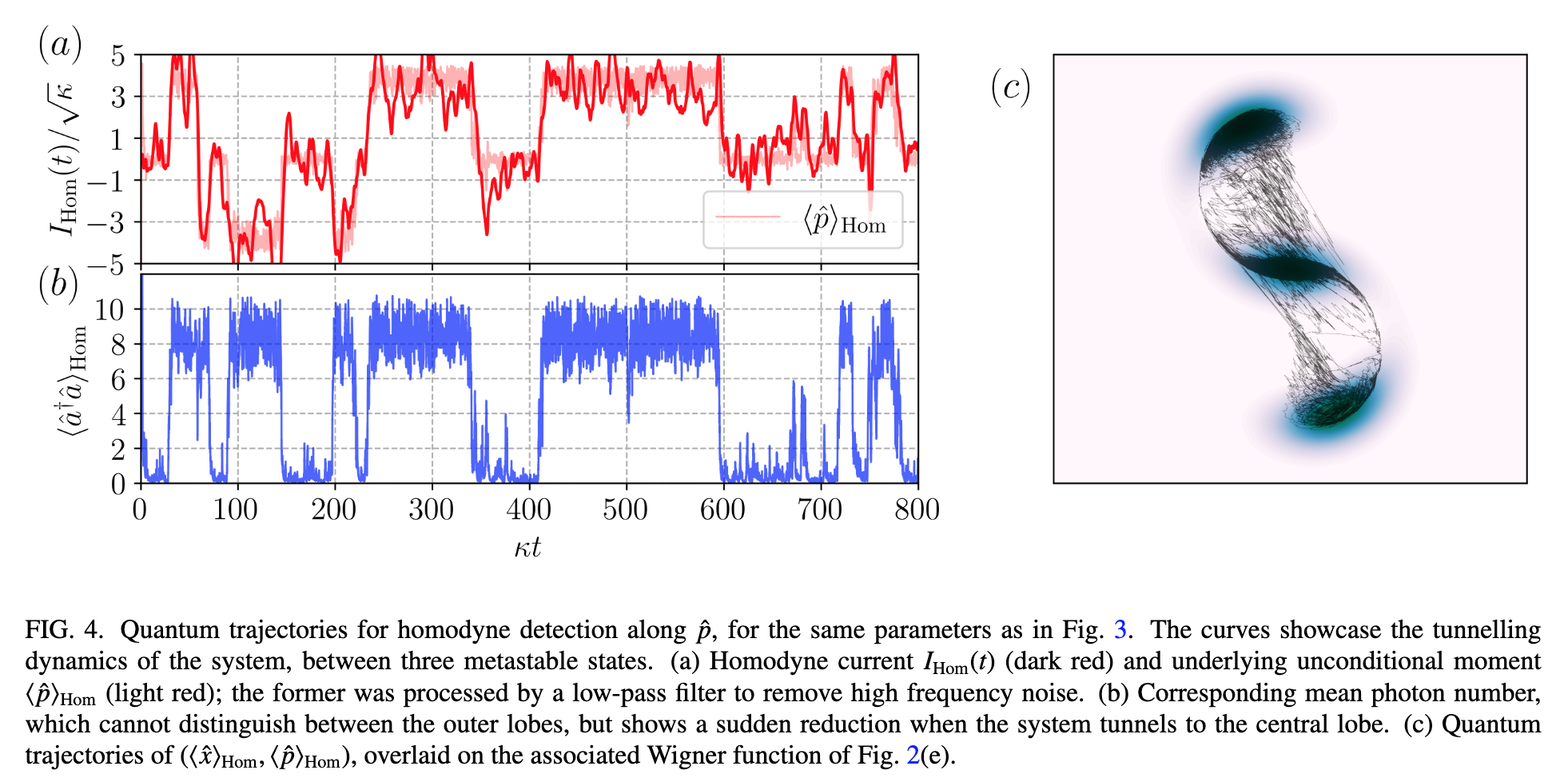
Reproduce Figures 1a, 1b, 2, 3a and 4c.

(Bonus) Extra challenge:

If there is time, reproduce also Fig. 5a (to get an exact match, \(N\) has to be chosen rather high especially for low \(U\), why? this results in high computation times, so for the sake of this exercise, I’d advise choosing \(N \approx 20\) and high \(U\) only). Implement equation (23). You may compare your results against the results produced using QuTiP built-in functions for solving master equations and computing Wigner functions. https://qutip.org/docs/4.0.2/guide/guide-correlation.html#steadystate-correlation-function